Databases store data in fixed-size pages (typically 8KB or 16KB), not as raw tables. Pages live in files on disk and get cached in a buffer pool in memory. Data is organized using B-trees for fast lookups. Before any write hits actual data, it goes to the Write-Ahead Log for crash recovery. Understanding this helps you write faster queries.
When you run a SQL query, something has to happen between your code and the spinning disk (or SSD) holding your data. Most developers treat this as a black box. The query goes in, data comes out. It works until it does not.
Understanding how databases actually store data changes how you think about performance. You will understand why some queries are fast and others are painfully slow. Why indexes matter. Why your database sometimes ignores the index you created. Why adding RAM helps more than adding CPU.
This guide walks through how databases store data, from the physical files on disk up to the memory structures that make everything fast. We will cover pages, B-trees, buffer pools, and write-ahead logs. The stuff that actually determines whether your app responds in 10 milliseconds or 10 seconds.
TL;DR: Databases store data in fixed-size pages (8-16KB blocks) organized into files on disk. Pages get cached in a buffer pool in memory. Data is organized using B-trees for fast lookups. All writes go to a Write-Ahead Log first for crash recovery. Row stores keep row data together (good for transactions). Column stores group column values (good for analytics).
The Journey of a Query
Before diving into storage details, here is the high-level picture of what happens when you run a query:
flowchart TD
    subgraph Client["fa:fa-user CLIENT"]
        SQL["SELECT * FROM users WHERE id = 1"]
    end

    Client ~~~ DBMS

    subgraph DBMS["fa:fa-database DATABASE ENGINE"]
        direction TB
        dbms_pad[ ]
        Parser["fa:fa-code Parser"]
        Optimizer["fa:fa-lightbulb Query Optimizer"]
        Executor["fa:fa-cogs Executor"]
        dbms_pad ~~~ Parser
    end

    subgraph Memory["fa:fa-memory MEMORY"]
        mem_pad[ ]
        BP["fa:fa-layer-group Buffer Pool"]
        mem_pad ~~~ BP
    end

    subgraph Storage["fa:fa-hdd DISK"]
        direction LR
        WAL["fa:fa-file-alt WAL"]
        DataFiles["fa:fa-folder Data Files"]
    end

    SQL --> Parser
    Parser --> Optimizer
    Optimizer --> Executor
    Executor --> BP
    BP -->|Cache Miss| DataFiles
    BP -->|Writes| WAL
    WAL -->|Checkpoint| DataFiles

    style Client fill:#e3f2fd,stroke:#1565c0,stroke-width:2px
    style DBMS fill:#fff3e0,stroke:#e65100,stroke-width:2px
    style Memory fill:#e8f5e9,stroke:#2e7d32,stroke-width:2px
    style Storage fill:#fce4ec,stroke:#c2185b,stroke-width:2px
    style dbms_pad fill:none,stroke:none,color:transparent
    style mem_pad fill:none,stroke:none,color:transparent
- Your SQL query gets parsed and optimized
- The executor figures out which data it needs
- It checks the buffer pool (memory cache) first
- If the data is not cached, it reads from disk files
- For writes, changes go to the Write-Ahead Log first
Now let us look at each layer in detail.
Pages: The Smallest Unit of Storage
Databases do not store data as rows or columns directly. They store data in fixed-size blocks called pages. This is the fundamental unit of storage.
| Database | Default Page Size |
|---|---|
| PostgreSQL | 8 KB |
| MySQL InnoDB | 16 KB |
| SQLite | 4 KB |
| SQL Server | 8 KB |
| Oracle | 8 KB |
When you query a single row, the database does not read just that row. It reads the entire page containing that row. When it writes a row, it writes the entire page.
Why pages? Because disk I/O is slow, but it gets faster when you read larger sequential blocks instead of tiny random chunks. Reading 8KB at once is almost as fast as reading 1 byte, but gives you far more data.
Page Structure
Every page has a consistent structure:
flowchart TB
    subgraph Page["fa:fa-file DATABASE PAGE 8KB"]
        direction TB
        subgraph Header["Page Header"]
            H1["Page ID"] --- H2["Page Type"] --- H3["Free Space Ptr"] --- H4["Checksum"]
        end
        subgraph Slots["Slot Array"]
            slots_pad[ ]
            S1["Slot 1"] --- S2["Slot 2"] --- S3["Slot 3"] --- S4["..."]
            slots_pad ~~~ S1
        end
        subgraph Free["Free Space"]
            free_pad[ ]
            F1[" "]
            free_pad ~~~ F1
        end
        subgraph Rows["Row Data"]
            rows_pad[ ]
            R3["Row 3"] --- R2["Row 2"] --- R1["Row 1"]
            rows_pad ~~~ R3
        end
    end

    Header --> Slots
    Slots --> Free
    Free --> Rows

    style Header fill:#e3f2fd,stroke:#1565c0,stroke-width:2px
    style Slots fill:#fff3e0,stroke:#e65100,stroke-width:2px
    style Free fill:#f5f5f5,stroke:#9e9e9e,stroke-width:2px
    style Rows fill:#e8f5e9,stroke:#2e7d32,stroke-width:2px
    style slots_pad fill:none,stroke:none,color:transparent
    style free_pad fill:none,stroke:none,color:transparent
    style rows_pad fill:none,stroke:none,color:transparent
Page Header: Metadata about the page including page ID, page type, free space pointers, checksum for detecting corruption, and transaction visibility information.
Slot Array: A directory that maps slot numbers to the actual position of each row within the page. This allows rows to be moved around within the page without changing their logical slot ID.
Free Space: Empty space in the middle of the page. Slots grow downward from the header, row data grows upward from the bottom.
Row Data: The actual tuples (rows), stored from the bottom of the page upward.
Slotted Pages: Handling Variable-Length Data
Most databases use a layout called slotted pages. The slot array at the top of the page contains pointers to where each row actually lives.
This design solves a tricky problem: rows have variable lengths. A VARCHAR column might hold 5 characters or 500. Without the slot array, deleting a row would leave a hole, and finding a row would require scanning from the start.
With slotted pages:
- The slot array always starts at the beginning (easy to find)
- Row data is appended from the end
- Deleting a row just marks its slot as empty
- Rows can be compacted without changing their slot ID
1
2
-- This query uses the slot array to find row location
SELECT * FROM users WHERE ctid = '(0,1)';  -- PostgreSQL: page 0, slot 1
In PostgreSQL, ctid exposes the physical location of a row as (page_number, slot_number). In MySQL InnoDB, rows are identified by their primary key value since InnoDB uses clustered indexes.
Heap vs Indexed Storage
Pages need to be organized somehow. There are two fundamental approaches:
Heap Storage
A heap is an unordered collection of pages. When you insert a row, the database finds any page with enough free space and puts it there. There is no particular order.
Finding a row in a heap: To find a specific row by some column value, you must scan every page. This is called a full table scan or sequential scan.
1
2
-- Without an index, this scans every page
SELECT * FROM users WHERE email = 'john@example.com';
For a table with 1 million rows spread across 100,000 pages, the database reads all 100,000 pages. Slow.
Indexed Storage (B-trees)
An index organizes data in a B-tree structure where rows (or pointers to rows) are sorted by the index key. Finding a row becomes a tree traversal instead of a full scan.
The B-tree keeps data sorted and balanced. Every search starts at the root and works down through intermediate nodes to the leaf nodes where the actual data (or data pointers) live.
flowchart TD
    subgraph BTree["B-Tree Index on user_id"]
        R["Root
50"]

        I1["25"]
        I2["75"]

        L1["10, 15, 20"]
        L2["30, 35, 40"]
        L3["55, 60, 65"]
        L4["80, 85, 90"]

        R --> I1
        R --> I2
        I1 --> L1
        I1 --> L2
        I2 --> L3
        I2 --> L4
    end

    style R fill:#e3f2fd,stroke:#1565c0,stroke-width:2px
    style I1 fill:#fff3e0,stroke:#e65100,stroke-width:2px
    style I2 fill:#fff3e0,stroke:#e65100,stroke-width:2px
    style L1 fill:#e8f5e9,stroke:#2e7d32,stroke-width:2px
    style L2 fill:#e8f5e9,stroke:#2e7d32,stroke-width:2px
    style L3 fill:#e8f5e9,stroke:#2e7d32,stroke-width:2px
    style L4 fill:#e8f5e9,stroke:#2e7d32,stroke-width:2px
To find user_id = 35:
- Start at root (50). 35 < 50, go left.
- At node 25. 35 > 25, go right.
- At leaf [30, 35, 40]. Found it.
Three page reads instead of 100,000. That is the power of B-trees.
For a deep dive into B-trees, see B-Tree Data Structure Explained.
Clustered vs Non-Clustered Indexes
Clustered Index: The leaf nodes of the B-tree contain the actual row data. The data is physically sorted by the index key. There can only be one clustered index per table because data can only be stored in one order.
Non-Clustered Index: The leaf nodes contain pointers (primary key values or row IDs) to the actual data. You need an extra lookup to get the row after finding it in the index.
| Feature | Clustered | Non-Clustered |
|---|---|---|
| Leaf nodes contain | Actual row data | Pointers to rows |
| Number per table | 1 | Many |
| Extra lookup needed | No | Yes |
| Range scans | Very fast | Slower |
In MySQL InnoDB, the primary key is always the clustered index. The actual table data lives in the B-tree organized by primary key. If you do not define a primary key, InnoDB creates a hidden one.
In PostgreSQL, tables are stored as heaps by default. Primary keys create a non-clustered index. You can optionally use CLUSTER to reorder heap data by an index, but this is a one-time operation, not automatically maintained.
1
2
3
4
5
6
7
8
9
10
11
12
13
-- MySQL: Primary key is clustered index
CREATE TABLE users (
    id INT PRIMARY KEY,    -- This becomes the clustered index
    email VARCHAR(255),
    name VARCHAR(100)
);

-- PostgreSQL: Create a separate index, data stored in heap
CREATE TABLE users (
    id SERIAL PRIMARY KEY,  -- Creates non-clustered index
    email VARCHAR(255),
    name VARCHAR(100)
);
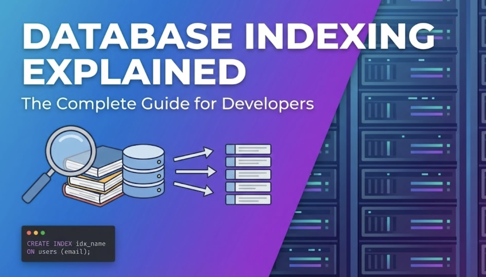
For more on indexing strategies, see How Database Indexing Works.
The Buffer Pool: Speed Through Caching
Disk access is slow. Memory access is fast. The buffer pool is how databases bridge this gap.
The buffer pool is an in-memory cache of pages. When you query data, the database first checks if the needed pages are already in the buffer pool. If yes, great. If not, it reads them from disk and caches them.
sequenceDiagram
    participant Q as Query
    participant BP as Buffer Pool (RAM)
    participant D as Data Files (Disk)

    Q->>BP: 1. Need page for user id=5
    alt Cache Hit
        BP-->>Q: Return cached page
    else Cache Miss
        BP->>D: 2. Read page from disk
        D-->>BP: 3. Return page
        BP->>BP: 4. Cache the page
        BP-->>Q: 5. Return data
    end
Why Not Let the OS Handle Caching?
Operating systems have their own file system cache. Why do databases need their own buffer pool?
Transaction safety: The database needs to control exactly when dirty pages (pages with unwritten changes) are flushed to disk. The OS flushes whenever it wants, potentially breaking crash recovery.
Eviction policies: The database knows which pages are likely to be needed soon based on query patterns. LRU (Least Recently Used) is not always optimal. The database might pin certain pages in memory or use more sophisticated eviction strategies.
Prefetching: When a query scans a range of data, the database can prefetch upcoming pages before they are needed. The OS does not know your query patterns.
Double caching: If both the OS and database cache pages, you waste memory storing the same data twice. Many databases bypass the OS cache using direct I/O (O_DIRECT on Linux).
Buffer Pool Configuration
The buffer pool is often the most important performance tuning parameter.
1
2
3
4
5
-- PostgreSQL: shared_buffers (typically 25% of RAM)
SHOW shared_buffers;

-- MySQL: innodb_buffer_pool_size (typically 70-80% of RAM)
SHOW VARIABLES LIKE 'innodb_buffer_pool_size';
A larger buffer pool means more pages can stay cached, reducing disk I/O. But you need to leave memory for the OS, query execution, connections, and other processes.
Monitoring Buffer Pool Hit Rate
A healthy database should have a high buffer pool hit rate (pages found in cache vs. pages read from disk).
1
2
3
4
5
6
7
8
9
-- PostgreSQL: Check hit rate
SELECT
    sum(heap_blks_hit) / (sum(heap_blks_hit) + sum(heap_blks_read)) AS hit_rate
FROM pg_statio_user_tables;

-- MySQL: Check buffer pool hit rate
SHOW STATUS LIKE 'Innodb_buffer_pool_read%';
-- Calculate: (Innodb_buffer_pool_read_requests - Innodb_buffer_pool_reads)
--            / Innodb_buffer_pool_read_requests
A hit rate below 99% often indicates you need more RAM or have inefficient queries scanning too much data.
Write-Ahead Log: The Safety Net
What happens if the power goes out while the database is writing data? Without protection, you could end up with partially written pages and corrupted data.
The Write-Ahead Log (WAL) solves this. Before any change is applied to actual data pages, it is first written to a sequential log file. Only after the log entry is safely on disk does the change get applied to the data pages.
sequenceDiagram
    participant App as Application
    participant BP as Buffer Pool
    participant WAL as Write-Ahead Log
    participant Data as Data Files

    App->>BP: UPDATE users SET name = 'Alice' WHERE id = 1
    BP->>BP: Modify page in memory (dirty page)
    BP->>WAL: Write log record: "Page X, offset Y, old value, new value"
    WAL-->>BP: Log record flushed to disk
    BP-->>App: Transaction committed

    Note over BP,Data: Later (checkpoint)
    BP->>Data: Write dirty pages to data files
Why This Order Matters
Crash before WAL write: Transaction not committed. No problem, nothing changed.
Crash after WAL write, before data page write: On restart, replay the WAL to redo the change. Data is consistent.
Crash after both writes: Everything fine.
The key insight: WAL writes are sequential (fast), while data page writes are random (slower). By writing sequentially to the WAL first, the database can acknowledge commits quickly. The slower random writes to data pages happen in the background.
| Database | WAL Name |
|---|---|
| PostgreSQL | Write-Ahead Log (WAL) |
| MySQL | Redo Log |
| SQL Server | Transaction Log |
| SQLite | Journal or WAL mode |
For a deeper explanation, see Write-Ahead Log: The Golden Rule of Durable Systems.
Checkpoints
Dirty pages in the buffer pool eventually need to be written to data files. This happens during checkpoints.
A checkpoint:
- Writes all dirty pages to data files
- Records the checkpoint position in the WAL
- Allows old WAL entries to be recycled
Checkpoints are expensive (lots of disk I/O) but necessary to bound recovery time. If the database never checkpointed, a crash would require replaying the entire WAL history.
1
2
3
4
5
-- PostgreSQL: Force a checkpoint (normally automatic)
CHECKPOINT;

-- See checkpoint activity
SELECT * FROM pg_stat_bgwriter;
Row Storage vs Column Storage
So far, we have discussed row-oriented storage where all columns of a row are stored together on the same page. This is how PostgreSQL, MySQL, Oracle, and most transactional databases work.
But there is another approach: column-oriented storage where all values for each column are stored together.
Row Store (Row-Oriented)
1
2
Page 1: [Row1: id=1, name="Alice", age=28] [Row2: id=2, name="Bob", age=35] ...
Page 2: [Row3: id=3, name="Carol", age=42] [Row4: id=4, name="Dave", age=31] ...
Good for: Reading full rows, inserting new rows, updating specific rows. Transactional workloads (OLTP).
Bad for: Aggregating a single column across millions of rows.
Column Store (Column-Oriented)
1
2
3
ID Column:   [1, 2, 3, 4, 5, ...]
Name Column: ["Alice", "Bob", "Carol", "Dave", ...]
Age Column:  [28, 35, 42, 31, ...]
Good for: Aggregating columns (SUM, AVG, COUNT), scanning large datasets. Analytical workloads (OLAP).
Bad for: Reading full rows, frequent updates.
When Column Stores Win
Say you want the average age of 10 million users:
1
SELECT AVG(age) FROM users;
Row store: Read all pages containing all columns (id, name, age, email, created_at, …) just to get the age column. Most of the data read is wasted.
Column store: Read only the age column pages. Much less I/O.
The performance difference can be 10x to 100x for analytical queries.
| Use Case | Better Choice |
|---|---|
| E-commerce transactions | Row store (PostgreSQL, MySQL) |
| User profile lookups | Row store |
| Sales analytics dashboard | Column store (ClickHouse, BigQuery) |
| Log aggregation | Column store |
| Real-time bidding | Row store |
| Business intelligence | Column store |
For more on this distinction, see Row vs Column Store Explained.
How Rows Are Identified Internally
Every row needs some way to be located. Different databases handle this differently.
PostgreSQL: ctid (Tuple ID)
PostgreSQL uses a hidden system column called ctid that stores (page_number, tuple_number). You can actually query it:
1
2
3
4
5
6
SELECT ctid, * FROM users LIMIT 5;
--  ctid  | id |  name
-- -------+----+--------
--  (0,1) |  1 | Alice
--  (0,2) |  2 | Bob
--  (0,3) |  3 | Carol
ctid = (0,1) means page 0, tuple 1.
Note: ctid values can change when rows are updated or the table is vacuumed. Do not use them as stable row identifiers.
MySQL InnoDB: Primary Key IS the Row Locator
In InnoDB, the primary key value is the row identifier. Data is stored in a clustered index sorted by primary key. Secondary indexes store the primary key value, not a physical location.
This is why primary key choice matters in MySQL. A large primary key (like a UUID) makes every secondary index larger because every leaf node stores a copy of the primary key.
1
2
3
4
-- MySQL: Secondary index lookups require two B-tree traversals
-- 1. Find primary key in secondary index
-- 2. Find row in clustered index using primary key
SELECT * FROM users WHERE email = 'alice@example.com';
Auto-Generated Row IDs
If you do not define a primary key:
PostgreSQL: Does not create one. Rows are identified by ctid (which can change).
MySQL InnoDB: Creates a hidden 6-byte row ID called DB_ROW_ID.
Always define an explicit primary key. Hidden row IDs work, but explicit primary keys give you more control and clarity.
Storage Manager: The Middleman
The storage manager is the component that translates logical operations (read page 123) into physical file operations. It maintains:
Page directory: Maps page IDs to file locations. Tracks which pages are allocated, which are free, and where new pages should go.
File organization: Decides how to split data across files. Some databases use one file per table. Others use tablespaces with multiple tables per file.
Space management: Tracks free space in each page. When inserting a row, finds a page with enough room.
1
2
3
4
5
6
-- PostgreSQL: See table file location
SELECT pg_relation_filepath('users');
-- Result: base/16384/16389

-- MySQL: Tables stored in data directory
-- /var/lib/mysql/mydb/users.ibd
MVCC: Reading Without Blocking Writes
Modern databases let readers and writers operate concurrently using Multi-Version Concurrency Control (MVCC).
Instead of locking rows when reading, the database keeps multiple versions of each row. Readers see a consistent snapshot based on their transaction start time, while writers create new versions.
PostgreSQL MVCC: Each row has hidden columns xmin (transaction that created it) and xmax (transaction that deleted/updated it). Old versions are kept in the same table until cleaned up by VACUUM.
MySQL InnoDB MVCC: Row versions are stored in the undo log. Old versions are reconstructed from the undo log when needed.
1
2
3
4
5
6
-- PostgreSQL: See MVCC columns
SELECT xmin, xmax, * FROM users LIMIT 3;
--  xmin  | xmax | id |  name
-- -------+------+----+--------
--  12345 |    0 |  1 | Alice   -- xmax=0 means row is current
--  12350 |    0 |  2 | Bob
This is why long-running transactions can cause problems. The database must keep old row versions around as long as any transaction might need them.
Putting It All Together
Here is the complete picture of how data flows through a typical database:
flowchart TB
    subgraph Client["fa:fa-user Application"]
        SQL["SQL Query"]
    end

    subgraph Engine["fa:fa-cogs Query Engine"]
        engine_pad[ ]
        Parser["Parser"]
        Optimizer["Optimizer"]
        Executor["Executor"]
        engine_pad ~~~ Parser
    end

    subgraph Memory["fa:fa-memory Memory Layer"]
        mem_pad[ ]
        BP["Buffer Pool
(Cached Pages)"]
        LC["Lock Manager"]
        mem_pad ~~~ BP
    end

    subgraph Storage["fa:fa-database Storage Layer"]
        storage_pad[ ]
        SM["Storage Manager"]
        WAL["Write-Ahead Log"]
        DF["Data Files
(Heap + Index Pages)"]
        storage_pad ~~~ SM
    end

    subgraph Disk["fa:fa-hdd Physical Storage"]
        disk_pad[ ]
        SSD["SSD/HDD"]
        disk_pad ~~~ SSD
    end

    SQL --> Parser
    Parser --> Optimizer
    Optimizer --> Executor
    Executor <--> BP
    Executor <--> LC
    BP <--> SM
    SM --> WAL
    SM <--> DF
    WAL --> SSD
    DF --> SSD

    style Client fill:#e3f2fd,stroke:#1565c0,stroke-width:2px
    style Engine fill:#fff3e0,stroke:#e65100,stroke-width:2px
    style Memory fill:#e8f5e9,stroke:#2e7d32,stroke-width:2px
    style Storage fill:#f3e5f5,stroke:#7b1fa2,stroke-width:2px
    style Disk fill:#fce4ec,stroke:#c2185b,stroke-width:2px
    style engine_pad fill:none,stroke:none,color:transparent
    style mem_pad fill:none,stroke:none,color:transparent
    style storage_pad fill:none,stroke:none,color:transparent
    style disk_pad fill:none,stroke:none,color:transparent
- Query comes in: Parsed, optimized, executed
- Executor needs data: Checks buffer pool
- Cache miss: Storage manager reads pages from data files
- Pages loaded: Cached in buffer pool, returned to executor
- Writes: Go to WAL first, then buffer pool marks pages dirty
- Checkpoints: Dirty pages written to data files
Practical Takeaways for Developers
Understanding database internals changes how you approach problems.
Why Indexes Matter
Without an index, finding a row means scanning every page. With an index, it is a B-tree traversal. The difference between O(n) and O(log n) is the difference between 10 seconds and 10 milliseconds.
Create indexes on columns used in WHERE, JOIN, and ORDER BY clauses. But do not over-index. Every index adds write overhead and storage cost.
Why RAM Helps More Than CPU
Most query time is spent waiting for disk I/O. More RAM means a larger buffer pool, more pages stay cached, fewer disk reads. Adding RAM often helps more than adding CPU cores.
Why Primary Key Choice Matters
In MySQL InnoDB, the primary key determines physical data order and is stored in every secondary index. Use small, sequential primary keys (INT or BIGINT) rather than large ones (UUID). See Snowflake ID Guide for generating sortable unique IDs.
Why Full Table Scans Are Expensive
A full table scan reads every page in the heap. For large tables, this means gigabytes of I/O even if you only need one row. Always check query plans for seq scans on large tables.
1
2
EXPLAIN ANALYZE SELECT * FROM users WHERE name = 'Alice';
-- Look for "Seq Scan" vs "Index Scan"
Why SELECT * Can Be Wasteful
Columns you do not need still get loaded from disk if they are on the same page as columns you do need. With covering indexes, fetching only indexed columns can skip the heap entirely.
1
2
-- With a covering index on (email, name), this never touches the heap
SELECT email, name FROM users WHERE email = 'alice@example.com';
Why Updates Are Expensive
Updates in PostgreSQL create a new row version and mark the old one deleted. The old version stays until VACUUM. Frequent updates cause table bloat and slow down scans.
In MySQL InnoDB, updates may require updating both the clustered index and every secondary index that includes the changed column.
Why SSDs Changed Everything
SSDs have much lower random read latency than spinning disks. This makes B-tree traversals faster and reduces the penalty of cache misses. If you are still on spinning disks, an SSD upgrade often helps more than any query tuning.
Further Reading
This post covered the fundamentals of database storage. Here are related topics to explore:
- PostgreSQL vs MongoDB vs DynamoDB: Which Should You Use in 2026? - Practical guide to picking the right database
- PostgreSQL Cheat Sheet - Practical commands, queries, and performance tuning for developers
- MongoDB Cheat Sheet - mongosh commands, aggregation pipeline, and indexing
- How Database Indexing Works - Deep dive into index types and query optimization
- Database Locks Explained - How locks, MVCC, and concurrency control work under the hood
- B-Tree Data Structure Explained - The data structure behind most indexes
- Write-Ahead Log Explained - How databases guarantee durability
- Row vs Column Store - Choosing the right storage model
- How OpenAI Scales PostgreSQL - Real-world scaling at massive scale
- Caching Strategies Explained - When the buffer pool is not enough
- Database Internals by Alex Petrov - Excellent book for going deeper
- Use The Index, Luke - Free resource on SQL indexing
Understanding how databases work helps you work with them, not against them. The next time a query is slow, you will know whether to add an index, increase the buffer pool, or rethink the query entirely.