What is the Fixed Partitions pattern in distributed systems?

Fixed Partitions is a data partitioning pattern that keeps the number of partitions constant for the life of the cluster. Keys are mapped to a fixed set of logical partitions using a hash, and those partitions are separately assigned to physical nodes. Because the partition count never changes, the key-to-partition mapping stays stable even as nodes are added or removed, so only whole partitions move during a resize instead of rehashing every key. It is documented in Unmesh Joshi's Patterns of Distributed Systems on Martin Fowler's site.

Why is hash(key) % nodeCount a bad way to distribute data?

Because the node count is part of the formula. The moment you add or remove a node, nodeCount changes, so the modulo result changes for almost every key, and nearly all data has to move to a different node. In a three-node cluster growing to five, the majority of keys get remapped. For large datasets this means a huge, slow, expensive data shuffle every time the cluster resizes, which defeats the point of scaling out smoothly.

What is the difference between Fixed Partitions and consistent hashing?

Both solve the same problem: keep data movement small when the cluster changes size. Fixed Partitions uses an explicit, fixed number of logical partitions (for example 1024) and a separate table that assigns partitions to nodes. Consistent hashing places nodes and keys on a hash ring and gives each node many virtual node positions to balance load. Fixed Partitions makes the partition count and ownership explicit and easy to reason about; consistent hashing avoids maintaining a large assignment table. Many systems blend the two ideas.

How many partitions should I choose?

Choose a number well above your expected maximum node count, so each node can hold several partitions and future nodes have partitions to receive, but not so high that per-partition overhead (metadata, open files, connections) becomes a burden. Common real-world choices are Redis Cluster's fixed 16384 hash slots and Kafka topics created with tens to hundreds of partitions. The key constraint is that changing the count later is expensive, so you size it once for future growth.

Can you change the number of partitions later?

It is possible but painful, which is the whole point of picking well up front. Changing the partition count changes the hash(key) % partitionCount result for most keys, so it triggers the same mass reshuffle that Fixed Partitions was meant to avoid. Kafka lets you increase a topic's partition count but warns that it breaks key-to-partition ordering guarantees. Redis Cluster keeps its 16384 slots fixed forever. Treat the partition count as a long-term decision, not a tuning knob.

Where is the partition-to-node mapping stored?

In a small, strongly consistent coordination service, often called a consistent core, such as ZooKeeper, etcd, or a Raft-based controller. Every client and node reads the same assignment table from there, so they all agree on which node currently owns each partition. When a rebalance moves a partition, the mapping is updated in one place and the change propagates to everyone, avoiding split views where two nodes think they own the same partition.

What is a hot partition and how does Fixed Partitions relate to it?

A hot partition is one that receives far more traffic than the others, usually because the partitioning key is skewed (for example, everything keyed by the same tenant or the same day). Fixed Partitions spreads keys across many partitions, which helps, but it cannot fix a bad key. If one key or a small key range dominates, its partition stays hot no matter how many partitions or nodes you have. Choosing a high-cardinality, evenly distributed partition key matters just as much as the pattern itself.

Fixed Partitions Pattern in Distributed Systems

Key Takeaways

Mapping keys directly to nodes with hash(key) % nodeCount is simple but brutal: change the node count and nearly every key moves to a different node.
Fixed Partitions adds a stable middle layer. Keys map to a fixed number of logical partitions; partitions map to nodes. Only the second mapping changes on a resize.
Because the partition count never changes, the key-to-partition math is stable, so rebalancing moves whole partitions, not individual keys.
Pick the partition count once, up front, and make it much larger than your expected node count. Changing it later is painful because it rehashes data.
The partition-to-node assignment lives in a consistent core like ZooKeeper or etcd, so every client and node agrees on who owns what.
Consistent hashing solves the same resize problem a different way. Fixed Partitions uses a fixed count of explicit partitions; consistent hashing uses a ring and virtual nodes.
Kafka, Redis Cluster, Cassandra, Akka Cluster Sharding, Hazelcast, and Ignite all lean on fixed partitions to scale horizontally without reshuffling everything.

Adding a server to a cluster should be boring. You slot in the new machine, it takes a share of the load, and life goes on. For a lot of naive data systems it is anything but boring, because the simple trick everyone reaches for first, hash(key) % numberOfNodes, has a nasty surprise built in: the moment the node count changes, almost every key wants to live on a different machine. Adding one node can trigger a shuffle of nearly all your data across the network.

The Fixed Partitions pattern is the fix, and it is one of the quietest, most important ideas behind every system that scales storage horizontally. The trick is to stop mapping keys straight to nodes. Instead you insert a stable layer in the middle: a fixed number of logical partitions that never changes. Keys map to partitions, and partitions map to nodes. When the cluster grows, you move whole partitions around, but no key ever gets rehashed.

This post walks through why the modulo approach breaks, how the fixed-partition layer works, what happens during a rebalance, how it compares to consistent hashing, how to pick the partition count, and how Kafka, Redis Cluster, Cassandra, and Akka all rely on it.

The Problem: Modulo Hashing Breaks on Resize

Say you are building a distributed key-value store, which is a good stand-in for most storage systems. You need to spread keys across a set of nodes with two goals:

Even distribution. No single node should get a wildly larger share than the others.
Cheap lookup. A client should know which node holds a key without asking every node.

The obvious answer is to hash the key and take it modulo the number of nodes. With three nodes, node = hash(key) % 3. It is fast, it needs no lookup table, and it spreads keys fairly evenly. Here is how a handful of keys land on a three-node cluster.

Key	hash(key) % 3	Node
Alice	0	Node 0
Bob	1	Node 1
Mary	2	Node 2
Philip	2	Node 2

Now the cluster gets busy and you add two more nodes, going from three to five. The formula is now hash(key) % 5, and the same keys land somewhere completely different.

Key	hash(key) % 5	Node
Alice	3	Node 3
Bob	1	Node 1
Mary	1	Node 1
Philip	1	Node 1

Look at what happened. Three of the four keys moved. Only Bob stayed put, and that was luck. The node count is baked right into the formula, so changing it changes the answer for almost every key. On a real cluster with terabytes of data, this means adding a single node triggers a mass migration where most of your data crosses the network to a new home.

flowchart TB
    subgraph before["fa:fa-server 3 nodes: node = hash(key) % 3"]
        direction LR
        K1["Alice"] --> N0["Node 0"]
        K2["Bob"] --> N1["Node 1"]
        K3["Mary"] --> N2["Node 2"]
        K4["Philip"] --> N2
    end

    subgraph after["fa:fa-server 5 nodes: node = hash(key) % 5"]
        direction LR
        A1["Alice"] --> M3["Node 3"]
        A2["Bob"] --> M1["Node 1"]
        A3["Mary"] --> M1
        A4["Philip"] --> M1
    end

    before ==>|"add 2 nodes"| after

    classDef key fill:#e0f2fe,stroke:#0891b2,stroke-width:2px,color:#0f172a
    classDef node fill:#dbeafe,stroke:#1d4ed8,stroke-width:2px,color:#0f172a
    classDef moved fill:#ffebee,stroke:#c62828,stroke-width:2px,color:#0f172a
    classDef lane fill:#f8fafc,stroke:#94a3b8,stroke-width:1px,color:#475569

    class K1,K2,K3,K4 key
    class N0,N1,N2 node
    class A1,A3,A4 moved
    class A2 key
    class M1,M3 node
    class before,after lane

The Solution: A Fixed Layer of Logical Partitions

The fix is a classic move in computer science: add a level of indirection. Instead of mapping keys directly to nodes, you map them to a fixed number of logical partitions, and then separately map partitions to nodes.

Keep the number of partitions fixed to keep the mapping of data to partition unchanged when the size of a cluster changes.

You launch the cluster with a preconfigured partition count, say 1024, and that number never changes for the life of the cluster. Because it is constant, the key-to-partition math, partition = hash(key) % 1024, always gives the same answer for the same key, no matter how many nodes you have. The only thing that changes when the cluster resizes is the second mapping: which node currently owns which partition.

%%{init: {'flowchart': {'curve': 'linear', 'nodeSpacing': 18, 'rankSpacing': 48}}}%%
flowchart LR
    Alice -->|"hash % 1024"| P12["Partition 12"] --> NA["Node A"]
    Bob -->|"hash % 1024"| P47["Partition 47"] --> NB["Node B"]
    Mary -->|"hash % 1024"| P883["Partition 883"] --> NC["Node C"]
    Philip -->|"hash % 1024"| P991["Partition 991"] --> NC

    classDef key fill:#e0f2fe,stroke:#0891b2,stroke-width:2px,color:#0f172a
    classDef part fill:#dbeafe,stroke:#1d4ed8,stroke-width:2px,color:#0f172a
    classDef node fill:#c8e6c9,stroke:#388e3c,stroke-width:2px,color:#0f172a

    class Alice,Bob,Mary,Philip key
    class P12,P47,P883,P991 part
    class NA,NB,NC node

The two mappings have very different lifetimes, and that is the whole idea:

Key to partition uses hash(key) % partitionCount. The count is fixed, so this mapping is permanent. A key belongs to the same partition forever.
Partition to node is an explicit assignment table. This is the flexible part. When nodes come and go, you edit this table, not the keys.

Because there are far more partitions than nodes, each node owns many partitions. A 1024-partition cluster running on 4 nodes gives each node about 256 partitions. Add a fifth node and you simply hand it roughly 205 partitions taken from the existing four. Only those partitions move. The 80 percent of data that was not in a moved partition stays exactly where it is.

How a Key Finds Its Node

Locating a key is now a two-step lookup, and both steps are cheap.

Compute the partition: partition = hash(key) % partitionCount. Pure math, no network call.
Look up which node owns that partition in the assignment table.

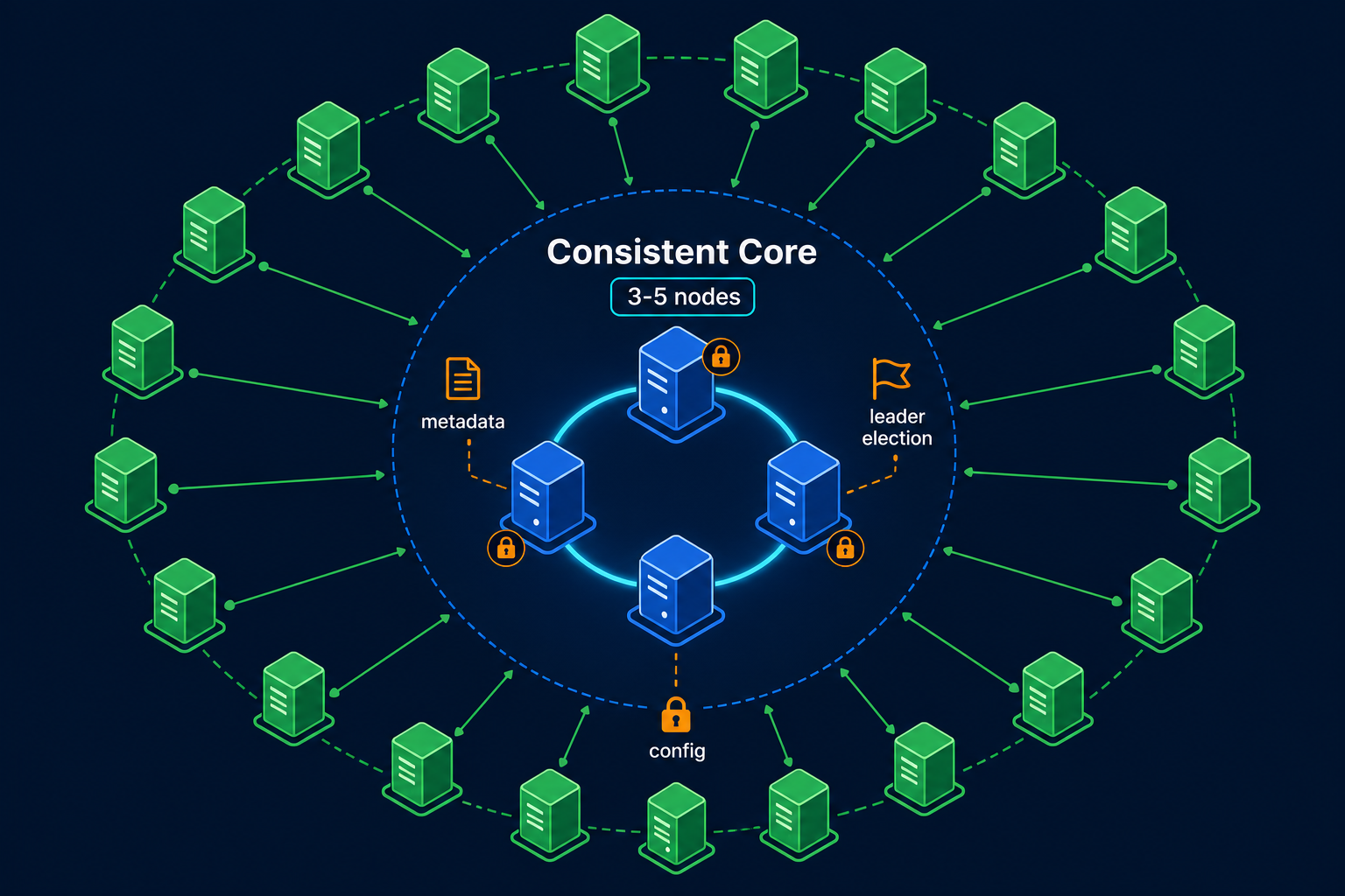
The assignment table is small, one row per partition, so it fits comfortably in memory and is easy to cache on every client. That table is the single source of truth for ownership, and it usually lives in a consistent core such as ZooKeeper or etcd so that every node and client sees the same view.

class PartitionedCluster:
    def __init__(self, partition_count):
        self.partition_count = partition_count      # fixed forever, e.g. 1024
        self.partition_to_node = {}                  # e.g. {0: "A", 1: "B", ...}

    def partition_for(self, key):
        # stable: same key always lands in the same partition
        return hash(key) % self.partition_count

    def node_for(self, key):
        partition = self.partition_for(key)
        return self.partition_to_node[partition]     # only this table changes on resize

    def reassign(self, partition, new_node):
        # rebalancing edits the table, it does not touch keys
        self.partition_to_node[partition] = new_node

Notice that partition_for never changes its behavior, while reassign is the only thing that runs during a rebalance. Keys are untouched. This clean split between a permanent hash and a mutable assignment table is the heart of the pattern.

Rebalancing: Move Partitions, Not Keys

Rebalancing is where the payoff shows up. When a node joins, leaves, or dies, the cluster wants partitions spread evenly again. With fixed partitions, rebalancing is a matter of reassigning some partitions and copying just their data, not rehashing the whole keyspace.

Here is what happens when a fourth node joins a three-node, twelve-partition cluster.

flowchart TB
    subgraph b["fa:fa-server Before: 3 nodes, 12 partitions (4 each)"]
        direction LR
        NA["Node A<br/>P0 P1 P2 P3"]
        NB["Node B<br/>P4 P5 P6 P7"]
        NC["Node C<br/>P8 P9 P10 P11"]
    end

    subgraph a["fa:fa-server After: 4 nodes, 12 partitions (3 each)"]
        direction LR
        NA2["Node A<br/>P0 P1 P2"]
        NB2["Node B<br/>P4 P5 P6"]
        NC2["Node C<br/>P8 P9 P10"]
        ND2["Node D<br/>P3 P7 P11"]
    end

    b ==>|"add Node D: move only P3, P7, P11"| a

    classDef node fill:#dbeafe,stroke:#1d4ed8,stroke-width:2px,color:#0f172a
    classDef newnode fill:#c8e6c9,stroke:#388e3c,stroke-width:2px,color:#0f172a
    classDef lane fill:#f8fafc,stroke:#94a3b8,stroke-width:1px,color:#475569

    class NA,NB,NC,NA2,NB2,NC2 node
    class ND2 newnode
    class b,a lane

More from Distributed systems

View All

Emergent Leader Pattern in Distributed Systems Aug 07, 2026

Request Waiting List Pattern in Distributed Systems Jul 24, 2026

Request Pipeline Pattern in Distributed Systems Jul 07, 2026

Consistent Core Pattern in Distributed Systems Jul 03, 2026

Leader and Followers Pattern in Distributed Systems Jun 16, 2026

Idempotent Receiver Pattern in Distributed Systems Jun 04, 2026

Only three partitions moved, one donated by each existing node, and the new node picked them up. Every other partition, and every key inside it, stayed exactly where it was. Compare that to modulo hashing, where adding the same node would have reshuffled the majority of keys. That is the difference between a five-minute rolling operation and an all-night data migration.

The mechanics of a safe partition move look like this:

The coordinator (or controller) decides partition P7 should move from Node B to the new Node D.
Node D starts copying P7’s data from Node B while Node B still serves reads and writes for it.
Once D has caught up, ownership flips in the assignment table, ideally guarded by a fencing token or version number so a stale node cannot keep serving the partition.
Clients refresh their cached assignment table and start routing P7’s traffic to Node D.

Because ownership changes are recorded in one authoritative place, the cluster avoids the split-brain nightmare where two nodes both think they own a partition. This is exactly why systems store the partition map in a consensus-backed store built on a replicated log.

Fixed Partitions vs Consistent Hashing

If you have read about consistent hashing, this all sounds familiar, because both patterns solve the same problem: keep data movement small when the cluster changes size. They just take different routes to get there.

Aspect	Fixed Partitions	Consistent Hashing
Core idea	A fixed count of explicit logical partitions	Nodes and keys placed on a hash ring
Key location	`hash(key) % partitionCount`, then a table lookup	First node clockwise on the ring
Ownership record	Explicit partition-to-node table	Ring positions, often with virtual nodes
On node change	Move a few whole partitions	Keys in the affected arc move
Balance control	Number of partitions per node	Number of virtual nodes per server
Reasoning	Very explicit, easy to inspect and rebalance	Elegant, but arcs can be uneven without vnodes
Used by	Kafka, Redis Cluster, Akka, Hazelcast, Ignite	DynamoDB, Cassandra, Memcached clients, many CDNs

The practical difference is how ownership is expressed. Fixed Partitions keeps an explicit table you can read, audit, and rebalance deliberately, which makes it easy to reason about and to move a specific partition to a specific node. Consistent hashing avoids maintaining a large table by deriving ownership from positions on a ring, using virtual nodes to smooth out the distribution. Interestingly, you can think of fixed partitions as consistent hashing where the “virtual nodes” are made concrete and given stable numbers. Many real systems blur the line: Cassandra’s vnodes are essentially a large, fixed set of token ranges, which is fixed partitioning wearing a ring.

How Many Partitions Should You Pick?

This is the one decision that really matters, because it is the hardest to change later. The partition count is a long-term commitment, so size it for the cluster you might have in a few years, not the one you have today.

Two forces pull in opposite directions:

Too few partitions and you cannot spread load well. If you have 8 partitions and want 12 nodes, four nodes sit idle with no partition to own. The partition count caps how far you can scale out.
Too many partitions and per-partition overhead adds up: metadata in the coordination service, open files, network connections, replication streams, and memory for each partition. Millions of partitions can overwhelm the control plane.

A good rule of thumb is to make the partition count comfortably larger than your maximum expected node count, so each node holds several partitions and there is always room to give new nodes work. Real systems bake in sensible defaults:

Redis Cluster fixes the count at 16384 hash slots, forever, for every cluster. Keys map to slots with CRC16(key) % 16384, and slots are assigned to nodes.
Kafka topics are created with a chosen partition count (often tens to low hundreds). You can increase it later, but doing so breaks per-key ordering, which is why teams try to get it right at creation.
Akka Cluster Sharding recommends a number of shards roughly ten times the maximum node count, for the same balance reasons.

The lesson across all of them is the same: choose once, choose generously, and treat the number as fixed.

The Pattern in Real Systems

Once you can name Fixed Partitions, you spot it in almost every horizontally scaled data system.

Apache Kafka

A Kafka topic is split into a fixed number of partitions chosen at creation. A record’s key decides its partition via hash(key) % partitionCount, and partitions are assigned to brokers. Adding brokers rebalances whole partitions across them without changing which partition a key belongs to. This is why Kafka can grow a cluster while preserving per-key ordering, and it is also why increasing partition count later is discouraged: it changes the key-to-partition mapping and breaks that ordering.

Redis Cluster

Redis Cluster is the textbook case. It defines exactly 16384 hash slots and never changes that number. Each master node owns a contiguous range of slots. Resharding means moving slots (and their keys) from one node to another while the slot count stays fixed. Clients cache the slot-to-node map and get redirected with MOVED or ASK responses when a slot has migrated.

Cassandra and DynamoDB

Both lean toward the consistent-hashing end of the spectrum, but the fixed-partition idea is still present. Cassandra splits the token ring into many virtual nodes (a large, effectively fixed set of token ranges) so that adding a node steals small ranges from many existing nodes rather than reshuffling everything. Amazon DynamoDB partitions data by the partition key and transparently splits partitions as data and traffic grow, keeping the key-to-partition mapping stable for clients.

Akka, Hazelcast, and Ignite

Actor and in-memory data grid frameworks use the pattern directly. Akka Cluster Sharding maps entities to a fixed number of shards, then distributes shards across the cluster. Hazelcast defaults to 271 partitions and Apache Ignite to 1024 by default, both fixed at startup, with backups of each partition placed on other nodes for fault tolerance.

System	Fixed unit	Typical count	Key to unit mapping
Kafka	Topic partition	Tens to hundreds	`hash(key) % partitions`
Redis Cluster	Hash slot	16384 (fixed)	`CRC16(key) % 16384`
Hazelcast	Partition	271 (default)	`hash(key) % 271`
Apache Ignite	Partition	1024 (default)	affinity function
Akka	Shard	~10x node count	`hash(entityId) % shards`

Trade-offs and When to Be Careful

Fixed Partitions is close to a free win for horizontal scaling, but it is not without edges.

What you gain:

Cheap resizing. Adding or removing nodes moves only a fraction of the data, so scaling is a routine operation instead of a scary migration.
Stable, cacheable lookups. The key-to-partition math never changes, and the small assignment table caches well on every client.
Explicit control. You can see exactly which node owns which partition and move specific partitions deliberately.

What it costs:

The count is a one-way door. Pick too low and you cap scale; pick too high and you drown the control plane. Changing it later triggers the very reshuffle you were avoiding.
You need a coordination service. The assignment table has to live somewhere strongly consistent, which means running or depending on a consistent core like ZooKeeper or etcd.
A bad key still bites. Fixed partitions spread keys, but if one key or key range is far hotter than the rest, its partition becomes a hot partition no matter how many partitions you have. Partition-key design matters as much as the pattern.
Rebalancing is not instant. Moving a partition means copying its data over the network while keeping it available, which takes time and bandwidth for large partitions.

Mistakes Teams Make

Using raw modulo hashing in the first place

The most common one. A quick prototype maps keys to nodes with hash(key) % nodeCount, it works fine in the demo, and then the first time the cluster scales in production it triggers a full data reshuffle. If your data is partitioned across nodes, reach for fixed partitions or consistent hashing from day one.

Setting the partition count too low

Teams often pick a partition count close to the current node count, “we have 4 nodes, let’s use 8 partitions.” Then growth stalls at 8 nodes because there are no spare partitions to hand out. Size the count for years of growth, not this quarter.

Setting the partition count absurdly high

The opposite error. Someone picks a million partitions “to be safe,” and the coordination service chokes on the metadata, or each node ends up managing tens of thousands of tiny partitions with real per-partition overhead. Pick generously, not infinitely.

Choosing a skewed partition key

Fixed partitions balance the number of keys, not the traffic. If you key by something low-cardinality or bursty, like a single popular tenant or the current calendar day, one partition gets hammered while the rest idle. A high-cardinality, evenly accessed key is what actually spreads load.

Letting clients act on a stale partition map

If a partition has moved but a client still routes to the old owner, you get errors or, worse, writes to the wrong node. Systems handle this with redirect responses (Redis MOVED/ASK) or version-checked assignments and fencing tokens. Do not assume every client instantly sees a rebalance.

Key Takeaways for Developers

Never map keys straight to nodes. hash(key) % nodeCount remaps almost everything the moment the node count changes. That is not a scaling strategy.
Add a fixed middle layer. Keys map to a fixed number of logical partitions; partitions map to nodes. Only the second mapping changes on a resize.
The partition count is permanent. The stability of the key-to-partition hash is the entire benefit, so treat the count as a long-term, hard-to-change decision.
Rebalancing moves partitions, not keys. Adding a node hands it a few whole partitions; everything else stays put.
Store the map in a consistent core. ZooKeeper, etcd, or a Raft controller keeps every client and node agreeing on who owns what.
Size the count for future growth. High enough that every node gets partitions and new nodes have work, low enough that the control plane stays healthy.
You already use it. Kafka, Redis Cluster, Cassandra, Akka, Hazelcast, and Ignite all scale on top of fixed partitions.

Wrapping Up

Fixed Partitions is a small idea with an outsized payoff. By refusing to bake the node count into how keys are located, and inserting a stable layer of logical partitions instead, you turn cluster resizing from a full-data migration into a quick move of a few partitions. The keys never rehash; only the partition-to-node table changes.

The wisdom is all in the details: pick the partition count generously and once, keep the assignment table in a strongly consistent store, guard ownership handoffs against stale nodes, and remember that a skewed key can still create a hot partition no matter how clever the pattern. Get those right and you have the same foundation that lets Kafka, Redis, and Cassandra grow from three nodes to three hundred without anyone losing a night’s sleep over a data shuffle.

Related posts:

Consistent Hashing Explained - The other main answer to the resize problem, using a ring instead of a fixed table
How Kafka Works - Topic partitions are fixed partitions in production
Consistent Core Pattern - Where the partition-to-node assignment table lives
Replicated Log - The consensus-backed log that records ownership changes safely
Leader and Followers Pattern - How each partition’s replicas stay in sync

Further reading: Unmesh Joshi’s Fixed Partitions chapter in Patterns of Distributed Systems; the Redis Cluster specification; the Akka Cluster Sharding docs; and the original Consistent Hashing paper by Karger et al.

Fixed Partitions Pattern in Distributed Systems

Why hashing keys straight to nodes falls apart when a cluster grows, and how a fixed layer of logical partitions keeps data movement small

The Problem: Modulo Hashing Breaks on Resize

Popular reads

The Solution: A Fixed Layer of Logical Partitions

How a Key Finds Its Node

Rebalancing: Move Partitions, Not Keys

More from Distributed systems

Fixed Partitions vs Consistent Hashing

How Many Partitions Should You Pick?

The Pattern in Real Systems

Apache Kafka

Redis Cluster

Cassandra and DynamoDB

Akka, Hazelcast, and Ignite

Trade-offs and When to Be Careful

Mistakes Teams Make

Using raw modulo hashing in the first place

Setting the partition count too low

Setting the partition count absurdly high

Choosing a skewed partition key

Letting clients act on a stale partition map

Key Takeaways for Developers

Wrapping Up

Subscribe via Email Always Free

More from Distributed systems

The Problem: Modulo Hashing Breaks on Resize

Popular reads

The Solution: A Fixed Layer of Logical Partitions

How a Key Finds Its Node

Rebalancing: Move Partitions, Not Keys

More from Distributed systems

Fixed Partitions vs Consistent Hashing

How Many Partitions Should You Pick?

The Pattern in Real Systems

Apache Kafka

Redis Cluster

Cassandra and DynamoDB

Akka, Hazelcast, and Ignite

Trade-offs and When to Be Careful

Mistakes Teams Make

Using raw modulo hashing in the first place

Setting the partition count too low

Setting the partition count absurdly high

Choosing a skewed partition key

Letting clients act on a stale partition map

Key Takeaways for Developers

Wrapping Up

Subscribe via Email Always Free

Share this:

Related Posts

More from Distributed systems